Gradient descent for smooth convex functions

Gradient descent uses local gradient information to reduce an objective function. To understand when this simple update works, we need to distinguish smoothness from convexity and examine what each assumption contributes.

This article develops the ideas in the following order: the meaning of smoothness, the quadratic error of a first-order approximation, the choice of step size, the convergence rate of gradient descent, quadratic upper bounds, optimality gaps, cocoercivity, and nonexpansiveness. A final connection explains why these ideas resemble the familiar fact that an orthogonal projection cannot increase the length of a segment.

Throughout, we work in Euclidean space. The notation $⟨u,v⟩=u^{\top }v$ denotes the inner product, and $\Vert \cdot {\Vert }_2$ denotes the Euclidean norm. The smoothness parameter $\beta$ is positive. Whenever a minimizer $x^{\ast }$ is used, we assume that a global minimizer exists. All optimization problems below are unconstrained unless a projection set is explicitly introduced.

---

1. What is a smooth function?

1.1 Smoothness in optimization

A differentiable function $f:{\mathbb{R}}^d\to \mathbb{R}$ is called $\beta$-smooth if its gradient is $\beta$-Lipschitz:

$$\Vert \nabla f(x)-\nabla f(y){\Vert }_2\le \beta \Vert x-y{\Vert }_2,x,y\in {\mathbb{R}}^d.$$

The slope cannot change arbitrarily abruptly. Moving the input by a distance $r$ changes the gradient by at most $\beta r$.

The definition requires differentiability. It also implies that the gradient is continuous. However, it does not require a second derivative to exist everywhere.

1.2 Classical smoothness and the notation C^k

In classical analysis, a smooth function usually means a function in $C^{\infty }$. The notation $C^k$ describes a class of functions; it is not an exponent applied to the function.

• $f\in C^0$: the function is continuous.
• $f\in C^1$: all first partial derivatives exist and are continuous.
• $f\in C^2$: all partial derivatives through order two exist and are continuous.
• $f\in C^k$: all partial derivatives through order $k$ exist and are continuous.
• $f\in C^{\infty }$: continuous partial derivatives exist at every order.

These classes are nested:

$$C^{\infty }\subseteq \cdots \subseteq C^2\subseteq C^1\subseteq C^0.$$

Classical smoothness and optimization smoothness are distinct notions. Neither implies the other globally, although both require differentiability.

For example, consider

$$f(x)=x|x|=\{\begin{array}{ll}{x}^2,& x\ge 0,\\ -x^2,& x<0.\end{array}$$

Its derivative is $f^{\prime }(x)=2|x|$, so

$$|f^{\prime }(x)-f^{\prime }(y)|=2||x|-|y||\le 2|x-y|.$$

Thus it is $2$-smooth. However, $f^{\prime \prime }(0)$ does not exist, so it belongs to $C^1$ but not $C^2$, and it is not classically smooth.

Conversely, $f(x)=x^4$ belongs to $C^{\infty }$, but it is not globally $\beta$-smooth for any finite $\beta$. Setting $y=0$ in the Lipschitz-gradient condition would require

$$4|x{|}^3\le \beta |x|,$$

or $4x^2\le \beta$ for every nonzero $x$, which is impossible. On a bounded interval $[-R,R]$, however, it is $12R^2$-smooth because $|f^{\prime \prime }(x)|=12x^2\le 12R^2$ there. The domain matters.

Finally, $f(x)=\cos x$ satisfies both notions. It is infinitely differentiable, and

$$|f^{\prime \prime }(x)|=|\cos x|\le 1,$$

so the mean value theorem gives $|f^{\prime }(x)-f^{\prime }(y)|\le |x-y|$. It is $1$-smooth on $\mathbb{R}$.

Function on the real line	Classically smooth?	Globally smooth in optimization?
$\cos x$	Yes	Yes, with $\beta =1$
$x^4$	Yes	No finite global smoothness constant
$x|x|$	No	Yes, with $\beta =2$

In the remainder of this article, “smooth” means smooth in the optimization sense.

---

2. First-order approximation has a controlled quadratic error

The first-order approximation of $f$ at a point $a$ is

$$f(y)\approx f(a)+⟨\nabla f(a),y-a⟩.$$

For a general differentiable function, this is a local approximation. Smoothness gives a quantitative error bound:

$$\boxed{\left|f(y)-f(x)-⟨\nabla f(x),y-x⟩\right|\le \frac{\beta }{2}\Vert y-x{\Vert }_2^2.}$$

In particular,

$$f(y)\le f(x)+⟨\nabla f(x),y-x⟩+\frac{\beta }{2}\Vert y-x{\Vert }_2^2.$$

2.1 Proof using the fundamental theorem of calculus

Set $h=y-x$ and define

$$\varphi (t)=f(x+th),0\le t\le 1.$$

Then $\varphi (0)=f(x)$, $\varphi (1)=f(y)$, and the chain rule gives

$${\varphi }^{\prime }(t)=⟨\nabla f(x+th),h⟩.$$

By the fundamental theorem of calculus,

$$f(y)-f(x)={\int }_0^1⟨\nabla f(x+th),h⟩dt.$$

Subtract the linear term:

$$f(y)-f(x)-⟨\nabla f(x),h⟩={\int }_0^1⟨\nabla f(x+th)-\nabla f(x),h⟩dt.$$

The expression on the left is the error of the first-order approximation. Using the triangle inequality, the Cauchy-Schwarz inequality, and smoothness, we obtain

$$\begin{array}{rl}\left|f(y)-f(x)-⟨\nabla f(x),h⟩\right|& \le {\int }_0^1\left|⟨\nabla f(x+th)-\nabla f(x),h⟩\right|dt\\ & \le {\int }_0^1\Vert \nabla f(x+th)-\nabla f(x){\Vert }_2\Vert h{\Vert }_{2}dt\\ & \le {\int }_0^1\beta t\Vert h{\Vert }_2^{2}dt\\ & =\frac{\beta }{2}\Vert h{\Vert }_2^2.\end{array}$$

Substituting $h=y-x$ proves the claim.

The quadratic dependence has a simple explanation: the gradient variation contributes one factor of $\Vert h{\Vert }_2$, and converting that variation into a function-value change contributes another. Integrating $t$ from zero to one produces the factor $1/2$.

This proof does not require convexity or the existence of a Hessian. The one-sided upper bound alone is not equivalent to Lipschitz continuity of the gradient for arbitrary nonconvex functions; the convex case will be discussed later.

---

3. Gradient descent and the role of the step size

Gradient descent updates the current point according to

$$x_{t+1}=x_t-{\eta }_t\nabla f(x_t),{\eta }_t>0.$$

The gradient points in the direction of greatest first-order increase under the Euclidean norm. Its negative therefore gives the direction of greatest first-order decrease.

In one variable, if $f^{\prime }(x_t)>0$, the update moves to the left. If $f^{\prime }(x_t)<0$, it moves to the right.

The aim is to reduce the objective and find a minimizer. For a general nonconvex function, gradient descent need not find a global minimum, and a zero gradient can also occur at a maximum or saddle point. Under convexity, every local minimum is global, and a zero gradient characterizes global optimality.

The step size controls how far we move:

• If it is too large, the update can pass the minimum, oscillate, or even increase the objective.
• If it is too small, each update makes little progress, and many iterations may be needed.

Passing the minimizer is not, by itself, a failure: an overshooting step can still decrease the function value. Smoothness tells us when a decrease is guaranteed.

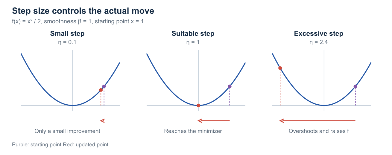
For the quadratic shown above, a tiny step moves only slightly; a suitable step makes useful progress; an excessively large step crosses the minimizer and increases the objective.

We use ${\eta }_t$ for the multiplier of the gradient throughout. The standard smoothness-based choice is ${\eta }_t=1/\beta$.

---

4. Smoothness and convexity are different assumptions

A function is convex if

$$f((1-s)x+sy)\le (1-s)f(x)+sf(y),0\le s\le 1.$$

Geometrically, its graph lies below the chord joining two points on the graph. For a differentiable function, convexity is equivalent to the first-order lower bound

$$f(y)\ge f(x)+⟨\nabla f(x),y-x⟩.$$

Smoothness and convexity do not imply one another.

4.1 Smooth but not convex: a negative quadratic

For $f(x)=-x^2$,

$$|f^{\prime }(x)-f^{\prime }(y)|=|-2x+2y|=2|x-y|.$$

It is $2$-smooth, but it curves downward and is not convex.

4.2 Convex but not smooth: absolute value

The function $f(x)=|x|$ is convex, but it is not differentiable at zero. Therefore, it is not $\beta$-smooth.

4.3 Smooth but not globally convex: cosine

The function $f(x)=\cos x$ is $1$-smooth, but its second derivative changes sign. It is not convex on all of $\mathbb{R}$.

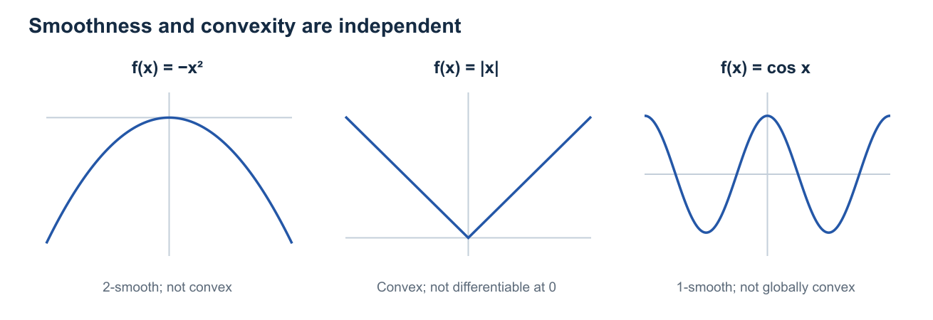
For a twice continuously differentiable function of one variable, the distinction is especially clear:

$$\begin{array}{rl}\text{Convexity:}& f^{\prime \prime }(x)\ge 0,\\ \beta \text{-smoothness:}& |f^{\prime \prime }(x)|\le \beta ,\\ \text{Both:}& 0\le f^{\prime \prime }(x)\le \beta .\end{array}$$

In several variables, the corresponding conditions use the Hessian:

$${\nabla }^{2}f(x)⪰0,\Vert {\nabla }^{2}f(x){\Vert }_{\mathrm{op}}\le \beta ,$$

and, when both hold,

$$0⪯{\nabla }^{2}f(x)⪯\beta I.$$

Convexity controls the sign of curvature; smoothness controls its magnitude.

---

5. Why a gradient step decreases the objective

Apply the quadratic upper bound with $x=x_t$ and $y=x_{t+1}$:

$$f(x_{t+1})\le f(x_t)+⟨\nabla f(x_t),x_{t+1}-x_t⟩+\frac{\beta }{2}\Vert x_{t+1}-x_t{\Vert }_2^2.$$

Since $x_{t+1}-x_t=-{\eta }_t\nabla f(x_t)$,

$$\begin{array}{rl}f(x_{t+1})& \le f(x_t)-{\eta }_t\Vert \nabla f(x_t){\Vert }_2^2+\frac{\beta {\eta }_t^2}{2}\Vert \nabla f(x_t){\Vert }_2^2\\ & =f(x_t)-{\eta }_t\left(1-\frac{\beta {\eta }_t}{2}\right)\Vert \nabla f(x_t){\Vert }_2^2.\end{array}$$

The linear approximation predicts a decrease. The quadratic term accounts for how much the actual function can depart from that approximation.

5.1 When is the decrease strict?

If

$$0<{\eta }_t<\frac{2}{\beta }\text{and}\nabla f(x_t)\ne 0,$$

then

$$f(x_{t+1})<f(x_t).$$

This decrease statement only requires smoothness. To replace “the gradient is nonzero” with “the point is not optimal,” we also use convexity. For a differentiable convex function on ${\mathbb{R}}^d$,

$$\nabla f(x)=0⟺x\text{ is a global minimizer}.$$

For a nonconvex example, $f(x)=\cos x$ has $f^{\prime }(0)=0$, but zero is a maximum. Gradient descent started there does not move.

5.2 Why choose the step size 1/beta?

The guaranteed decrease coefficient is

$$\eta -\frac{\beta {\eta }^2}{2}=\frac{1}{2\beta }-\frac{\beta }{2}{\left(\eta -\frac{1}{\beta }\right)}^2.$$

It is maximized at $\eta =1/\beta$. Equivalently, the coefficient $-\eta +\beta {\eta }^2/2$ in the upper bound is minimized there. Thus

$$\boxed{f(x_{t+1})\le f(x_t)-\frac{1}{2\beta }\Vert \nabla f(x_t){\Vert }_2^2.}$$

This choice optimizes the decrease guaranteed by the smoothness bound. It need not minimize the actual function along the search direction.

---

6. Convergence rate of gradient descent

6.1 The theorem

Suppose $f:{\mathbb{R}}^d\to \mathbb{R}$ is convex and $\beta$-smooth, and a minimizer $x^{\ast }$ exists. Run gradient descent with

$$x_{t+1}=x_t-\frac{1}{\beta }\nabla f(x_t).$$

After $T$ updates starting from $x_1$,

$$\boxed{f(x_{T+1})-f(x^{\ast })\le \frac{\beta \Vert x_1-x^{\ast }{\Vert }_2^2}{2T}.}$$

This theorem bounds the error in the function value, not directly the distance between the iterate and a minimizer.

6.2 Combine smoothness and convexity

The decrease inequality gives

$$f(x_{t+1})\le f(x_t)-\frac{1}{2\beta }\Vert \nabla f(x_t){\Vert }_2^2.$$

Convexity gives

$$f(x^{\ast })\ge f(x_t)+⟨\nabla f(x_t),x^{\ast }-x_t⟩.$$

Writing $g_t=\nabla f(x_t)$ and combining the inequalities,

$$f(x_{t+1})-f(x^{\ast })\le ⟨g_t,x_t-x^{\ast }⟩-\frac{1}{2\beta }\Vert g_t{\Vert }_2^2.$$

6.3 Express the bound as a change in squared distance

Recall the identity

$$\Vert a-b{\Vert }_2^2=\Vert a{\Vert }_2^2-2⟨a,b⟩+\Vert b{\Vert }_2^2.$$

Using the gradient update,

$$\begin{array}{rl}\Vert x_{t+1}-x^{\ast }{\Vert }_2^2& ={\Vert x_t-x^{\ast }-\frac{1}{\beta }{g}_t\Vert }_2^2\\ & =\Vert x_t-x^{\ast }{\Vert }_2^2-\frac{2}{\beta }⟨g_t,x_t-x^{\ast }⟩+\frac{1}{{\beta }^2}\Vert g_t{\Vert }_2^2.\end{array}$$

Rearranging yields

$$⟨g_t,x_t-x^{\ast }⟩-\frac{1}{2\beta }\Vert g_t{\Vert }_2^2=\frac{\beta }{2}\left(\Vert x_t-x^{\ast }{\Vert }_2^2-\Vert x_{t+1}-x^{\ast }{\Vert }_2^2\right).$$

Therefore,

$$f(x_{t+1})-f(x^{\ast })\le \frac{\beta }{2}\left(\Vert x_t-x^{\ast }{\Vert }_2^2-\Vert x_{t+1}-x^{\ast }{\Vert }_2^2\right).$$

The remaining function-value error is bounded by the reduction in squared distance, multiplied by $\beta /2$.

6.4 Sum and telescope

Let $D_t=\Vert x_t-x^{\ast }{\Vert }_2^2$. Summing over $t=1,\dots ,T$ gives

$$\begin{array}{rl}\sum _{t=1}^T(f(x_{t+1})-f(x^{\ast }))& \le \frac{\beta }{2}\sum _{t=1}^T(D_t-D_{t+1})\\ & =\frac{\beta }{2}(D_1-D_{T+1})\\ & \le \frac{\beta }{2}{D}_1.\end{array}$$

All intermediate distance terms cancel. Dividing by $T$,

$$\frac{1}{T}\sum _{t=1}^T(f(x_{t+1})-f(x^{\ast }))\le \frac{\beta }{2T}\Vert x_1-x^{\ast }{\Vert }_2^2.$$

6.5 Pass from the average error to the last iterate

The function values are nonincreasing:

$$f(x_2)\ge f(x_3)\ge \cdots \ge f(x_{T+1}).$$

The last value is no larger than their average. Consequently,

$$\begin{array}{rl}f(x_{T+1})-f(x^{\ast })& \le \frac{1}{T}\sum _{t=1}^T(f(x_{t+1})-f(x^{\ast }))\\ & \le \frac{\beta \Vert x_1-x^{\ast }{\Vert }_2^2}{2T}.\end{array}$$

This completes the proof. The algorithm may return the last iterate; averaging the iterates is not required for this guarantee.

6.6 What does O(1/T) mean?

Write

$$E_T=f(x_{T+1})-f(x^{\ast }),C=\frac{\beta }{2}\Vert x_1-x^{\ast }{\Vert }_2^2.$$

The theorem states $E_T\le C/T$. With $\beta$ and the initial distance fixed, we express this as

$$E_T=O(1/T).$$

Big O describes an upper-bound scaling while suppressing fixed multiplicative constants. Ten times as many iterations makes this error bound ten times smaller. It does not assert that the actual error decreases by exactly that factor.

For example, if $C=10$:

Number of updates	Guaranteed error bound
$10$	$1$
$100$	$0.1$
$1000$	$0.01$

If the target error is $ϵ>0$, it suffices to ensure

$$\frac{C}{T}\le ϵ,\text{or equivalently}T\ge \frac{C}{ϵ}.$$

Choosing an integer number of updates at least this large gives an iteration complexity of

$$O(1/ϵ).$$

The two statements answer different questions: $O(1/T)$ bounds the error given a number of steps, while $O(1/ϵ)$ bounds the work sufficient for a target accuracy.

6.7 Constant step size and the self-tuning property

The step size $\eta =1/\beta$ is constant and does not depend on $T$. Nevertheless, the actual movement is

$$\Vert x_{t+1}-x_t{\Vert }_2=\frac{1}{\beta }\Vert \nabla f(x_t){\Vert }_2.$$

As the gradient approaches zero, the movement approaches zero automatically. The constant step size and the actual displacement are different quantities. This automatic adjustment is the self-tuning property described in the notes.

6.8 Comparison with the subgradient method

For a convex objective whose subgradients have norm at most $L$, a standard constant-step subgradient analysis gives, with $R=\Vert x_1-x^{\ast }{\Vert }_2$,

$$f\left(\frac{1}{T}\sum _{t=1}^T{x}_t\right)-f(x^{\ast })\le \frac{1}{T}\sum _{t=1}^T(f(x_t)-f(x^{\ast }))\le \frac{R^2}{2\eta T}+\frac{\eta L^2}{2}.$$

Here the first inequality follows from convexity. For positive $R$ and $L$, choosing $\eta =R/(L\sqrt{T})$ balances the two terms and yields an $O(1/\sqrt{T})$ error guarantee, or $O(1/{ϵ}^2)$ iterations for accuracy $ϵ$.

The smooth analysis has no residual term $\eta L^2/2$. With $\eta =1/\beta$,

$$f(x_{T+1})-f(x^{\ast })\le \frac{R^2}{2\eta T}.$$

Smoothness permits a constant step size independent of the iteration budget and guarantees that the last iterate is no worse than the average function value. Nonsmooth subgradient steps do not generally decrease the objective at every iteration.

---

7. Quadratic upper bounds and their geometric meaning

For a convex, smooth function, convexity and smoothness together give

$$\boxed{f(x)+⟨\nabla f(x),y-x⟩\le f(y)\le f(x)+⟨\nabla f(x),y-x⟩+\frac{\beta }{2}\Vert y-x{\Vert }_2^2.}$$

The first-order model is a lower bound. Adding the quadratic correction gives an upper bound. Both models agree with $f$ at the current point $x$.

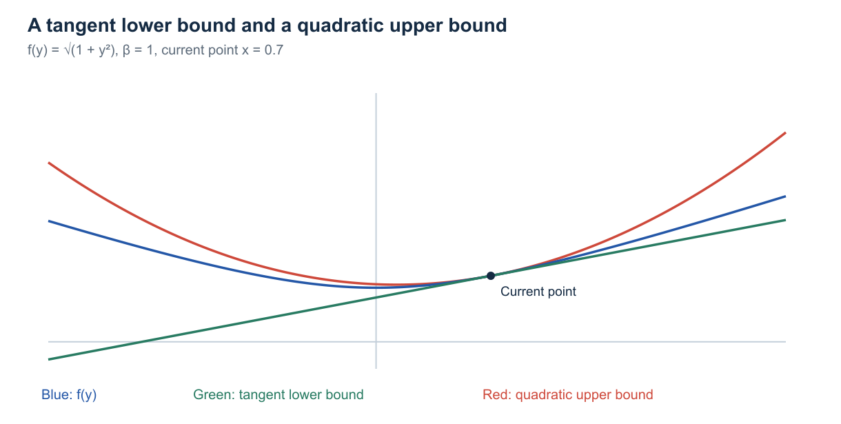
The tangent line lies below the function, while the quadratic model lies above it. Both touch the function at the current point.

7.1 An equivalent convexity characterization

For a differentiable convex function $f$, the following are equivalent:

$$f\text{ is }\beta \text{-smooth}⟺q(x)=\frac{\beta }{2}\Vert x{\Vert }_2^2-f(x)\text{ is convex}.$$

In one dimension, if a continuous second derivative exists,

$$q^{\prime \prime }(x)=\beta -f^{\prime \prime }(x).$$

Convexity of both $f$ and $q$ means $0\le f^{\prime \prime }(x)\le \beta$. The reference quadratic has enough curvature that subtracting $f$ leaves a convex function. The characterization remains valid without assuming a second derivative exists.

To see the forward direction, note that

$$\begin{array}{rl}⟨\nabla q(x)-\nabla q(y),x-y⟩& =\beta \Vert x-y{\Vert }_2^2-⟨\nabla f(x)-\nabla f(y),x-y⟩\\ & \ge 0,\end{array}$$

where Cauchy-Schwarz and smoothness give the final inequality. A differentiable function with a monotone gradient is convex.

For the reverse direction, convexity of $q$ gives

$$\frac{\beta }{2}\Vert z{\Vert }_2^2-f(z)\ge \frac{\beta }{2}\Vert x{\Vert }_2^2-f(x)+⟨\beta x-\nabla f(x),z-x⟩.$$

Rearranging produces the quadratic upper bound for $f$. To recover the Lipschitz-gradient condition, set

$$\Delta =\nabla f(x)-\nabla f(y),z=y+\frac{1}{\beta }\Delta .$$

Combining the convex lower bound at $x$ with the quadratic upper bound at $y$,

$$\begin{array}{rl}f(x)-f(y)& =f(x)-f(z)+f(z)-f(y)\\ & \le ⟨\nabla f(x),x-z⟩+⟨\nabla f(y),z-y⟩+\frac{\beta }{2}\Vert z-y{\Vert }_2^2\\ & =⟨\nabla f(x),x-y⟩-\frac{1}{2\beta }\Vert \Delta {\Vert }_2^2.\end{array}$$

Swap $x$ and $y$ and add the two inequalities. Then

$$\frac{1}{\beta }\Vert \Delta {\Vert }_2^2\le ⟨\Delta ,x-y⟩\le \Vert \Delta {\Vert }_2\Vert x-y{\Vert }_2.$$

If $\Delta =0$, the desired bound is immediate. Otherwise, divide by $\Vert \Delta {\Vert }_2$ to obtain

$$\Vert \nabla f(x)-\nabla f(y){\Vert }_2\le \beta \Vert x-y{\Vert }_2.$$

7.2 Gradient descent minimizes a touching quadratic upper bound

At the current point $x$, define

$$Q_x(y)=f(x)+⟨\nabla f(x),y-x⟩+\frac{\beta }{2}\Vert y-x{\Vert }_2^2.$$

Although minimizing $f$ directly may be difficult, minimizing $Q_x$ is easy:

$${\nabla }_y{Q}_x(y)=\nabla f(x)+\beta (y-x)=0$$

gives

$$y=x-\frac{1}{\beta }\nabla f(x).$$

Thus each gradient-descent step minimizes a quadratic upper bound touching the function at the current point. Since $Q_x(x)=f(x)$,

$$f(x^{+})\le Q_x(x^{+})\le Q_x(x)=f(x),x^{+}=x-\frac{1}{\beta }\nabla f(x).$$

This explains both the update and the step size geometrically.

---

8. Optimality gaps: function values, gradients, and distances

8.1 The theorem

For a convex, $\beta$-smooth function with a minimizer $x^{\ast }$,

$$\boxed{\frac{1}{2\beta }\Vert \nabla f(x){\Vert }_2^2\le f(x)-f(x^{\ast })\le \frac{\beta }{2}\Vert x-x^{\ast }{\Vert }_2^2.}$$

The middle expression is an error in function value, not an error in the location $x$.

8.2 Proof of the upper bound

Apply the quadratic upper bound at $x^{\ast }$:

$$f(x)\le f(x^{\ast })+⟨\nabla f(x^{\ast }),x-x^{\ast }⟩+\frac{\beta }{2}\Vert x-x^{\ast }{\Vert }_2^2.$$

Because $\nabla f(x^{\ast })=0$,

$$f(x)-f(x^{\ast })\le \frac{\beta }{2}\Vert x-x^{\ast }{\Vert }_2^2.$$

This converts a guarantee about location into a guarantee about objective value. If $\Vert x-x^{\ast }{\Vert }_2\le r$, then the gap is at most $\beta r^2/2$.

8.3 Proof of the lower bound

Take one gradient step,

$$y=x-\frac{1}{\beta }\nabla f(x).$$

Global optimality of $x^{\ast }$ and the decrease inequality imply

$$f(x^{\ast })\le f(y)\le f(x)-\frac{1}{2\beta }\Vert \nabla f(x){\Vert }_2^2.$$

Rearranging gives the lower bound.

The gap to the minimum must be at least as large as the decrease guaranteed by one gradient step.

8.4 What the theorem does and does not guarantee

• Being close to a minimizer guarantees a small function-value gap.
• A large gradient implies a gap at least as large as the stated lower bound.
• A small gap implies a small gradient.
• A small gradient alone does not guarantee a small gap under these assumptions.

For example, let $0<\delta \le 1$ and consider the convex, $1$-smooth function

$$f(u,v)=\frac{1}{2}{u}^2+\frac{\delta }{2}{v}^2.$$

At $(u,v)=(0,1/\sqrt{\delta })$,

$$f(u,v)-f(0,0)=\frac{1}{2},\Vert \nabla f(u,v){\Vert }_2=\sqrt{\delta }.$$

The gradient can be arbitrarily small across this family while the gap remains $1/2$. An upper bound on the gap based only on the gradient requires additional information, such as a strong-convexity parameter.

---

9. Cocoercivity of the gradient

For a convex, $\beta$-smooth function,

$$\boxed{⟨\nabla f(x)-\nabla f(y),x-y⟩\ge \frac{1}{\beta }\Vert \nabla f(x)-\nabla f(y){\Vert }_2^2.}$$

This property is called cocoercivity. It relates the change in gradients to the change in positions.

Convexity alone gives a nonnegative inner product. Smoothness strengthens this to a quantitative positive alignment whenever the gradients differ. The two vectors need not point in exactly the same direction.

9.1 Proof using the optimality-gap bound

Fix $x,y$ and define functions of a new variable $z$:

$$g(z)=f(z)-⟨\nabla f(x),z⟩,h(z)=f(z)-⟨\nabla f(y),z⟩.$$

Subtracting a linear function preserves convexity and does not change gradient differences, so both functions are convex and $\beta$-smooth. Their gradients are

$$\nabla g(z)=\nabla f(z)-\nabla f(x),\nabla h(z)=\nabla f(z)-\nabla f(y).$$

Thus $\nabla g(x)=0$ and $\nabla h(y)=0$. By convexity, $x$ minimizes $g$ and $y$ minimizes $h$.

Apply the lower optimality-gap bound to $g$ at $y$:

$$\begin{array}{rl}f(y)-f(x)-⟨\nabla f(x),y-x⟩& =g(y)-g(x)\\ & \ge \frac{1}{2\beta }\Vert \nabla g(y){\Vert }_2^2\\ & =\frac{1}{2\beta }\Vert \nabla f(y)-\nabla f(x){\Vert }_2^2.\end{array}$$

Similarly, apply it to $h$ at $x$:

$$f(x)-f(y)-⟨\nabla f(y),x-y⟩\ge \frac{1}{2\beta }\Vert \nabla f(x)-\nabla f(y){\Vert }_2^2.$$

Adding the inequalities cancels the function values and gives

$$⟨\nabla f(x)-\nabla f(y),x-y⟩\ge \frac{1}{\beta }\Vert \nabla f(x)-\nabla f(y){\Vert }_2^2.$$

This is the same strengthened gradient inequality encountered in the convexity characterization of smoothness.

---

10. Nonexpansiveness of the gradient-descent update

Define the update map

$$G(x)=x-\frac{1}{\beta }\nabla f(x).$$

For a convex, $\beta$-smooth function, this map is nonexpansive:

$$\boxed{\Vert G(x)-G(y){\Vert }_2\le \Vert x-y{\Vert }_2.}$$

If we start at two different points and apply the same gradient-descent update, the distance between the resulting points does not increase.

10.1 Proof

Let

$$d=x-y,\Delta =\nabla f(x)-\nabla f(y).$$

Then

$$\begin{array}{rl}\Vert G(x)-G(y){\Vert }_2^2& ={\Vert d-\frac{1}{\beta }\Delta \Vert }_2^2\\ & =\Vert d{\Vert }_2^2-\frac{2}{\beta }⟨d,\Delta ⟩+\frac{1}{{\beta }^2}\Vert \Delta {\Vert }_2^2\\ & \le \Vert d{\Vert }_2^2-\frac{1}{{\beta }^2}\Vert \Delta {\Vert }_2^2\\ & \le \Vert d{\Vert }_2^2.\end{array}$$

The first inequality uses cocoercivity. Taking square roots proves the claim.

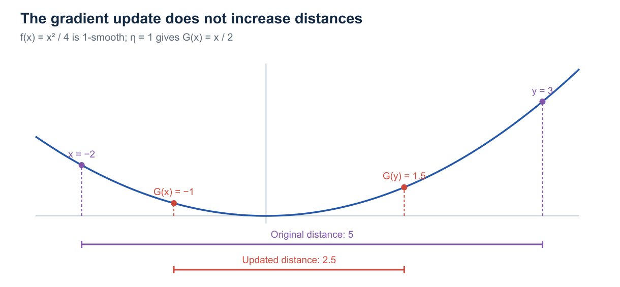
The two starting points are shown in purple, and their updated positions in red. Horizontal distances represent distances between inputs. This example contracts the distance; the general theorem only guarantees that the distance does not increase.

10.2 Why this property matters

Nonexpansiveness is a stability statement: differences in starting points are not amplified by one update. Repeating the inequality shows that two trajectories using this same update satisfy

$$\Vert x_t-y_t{\Vert }_2\le \Vert x_1-y_1{\Vert }_2.$$

In particular, a minimizer satisfies $G(x^{\ast })=x^{\ast }$. Setting $y=x^{\ast }$ gives

$$\Vert x_{t+1}-x^{\ast }{\Vert }_2\le \Vert x_t-x^{\ast }{\Vert }_2.$$

The distance to a minimizer does not increase. Nonexpansiveness alone does not imply a fixed percentage of shrinkage at every step, uniqueness of the minimizer, or a geometric convergence rate.